Asset allocation
This chapters shows how to allocate financial instruments.
├── Expected return
│   ├── ...
│   └── ...
├── Risk estimation
│   ├── Volatility
│   └── Correlation
├── Portfolio optimization
│   ├── Mean-Variance
│   ├── Black-Litterman
│   ├── DP(Dynamic Programming)
└── └── RO(Robust Optimization)
Expected return
Risk estimation
Volatility
Correlation
Portfolio optimization
Mean-Variance
Black-Litterman
본 내용은 ‘A step by step guide to Black-Litterman Model(2002)’을 기반으로 작성하였습니다.
Black Litterman 모델은 1990년 골드만삭스의 피셔블랙(Fischer Black)과 로버트 리터만(Robert Litterman)에 의해 개발된 포트폴리오 배분을 위한 수학적 모형이다. 이 모형은 자산배분이 가능한 모든 자산은 시장가치에 비례한다는 균형가정 (Equilibruim)과 투자자의 시장전망 (View)를 고려하여 맞춤식 자산배분이 가능하다. 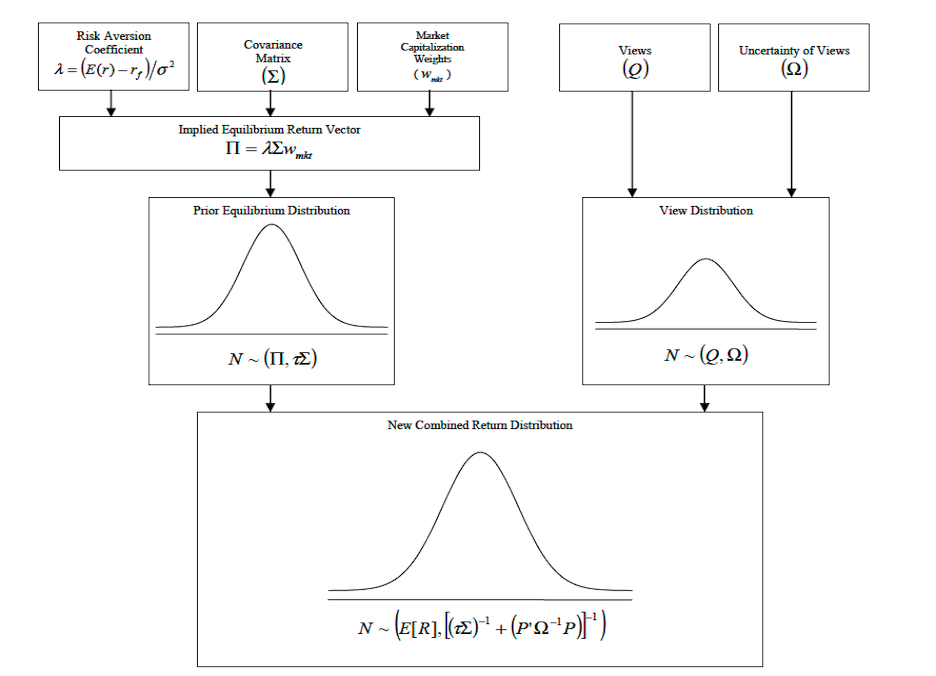
블랙리터만모형은 베이지안 통계에 기반하여 시장에서의 정보(Implied Equilibrium Return)와 수익률에 대한 투자자의 전망(Investor’s View)을 결합하여 새로운 기대수익률(New Combined Expected Return)을 도출한다.
- Black-Litterman Formula
\(E[R] =[(\tau\Sigma)^{-1} + P'\Omega^{-1} P]^{-1} [(\tau\Sigma)^-1 + P'\Omega^{-1} Q]\)\(\tau\) : risk adjustment scalar
\(\Sigma\) : Covariance Matrix of excess returns
\(P\) : Matrix that identifies the asset involved in the views
\(Q\) : View Vector
\(\Omega\) : diagonal covariance matrix of view’s error terms - Calculate Equilibrium Return
블랙 리터만 모형의 첫 번째 과정은 시장 포트폴리오 비율로부터 시장에 내재되어있는 기대수익률을 계산한다.
역최적화(inverse optimization)을 통하여 기대수익률에 대한 시장의 분포를 도출하기 위한 과정이다.- Implied Equilibrium Return
\(\Pi = \lambda\Sigma w_{mkt}\)\(w_{mkt}\) : Market capitalization weights
\(\lambda\) : Risk aversion, \(\lambda = {(E(r) - r_f)\over \sigma^2}\)
\(\Sigma\) : Covariance matrix
- Implied Equilibrium Return
- Investor’s View
블랙 리터만 모형은 투자자의 전망을 결합하여 자산배분 비율을 결정하는 모형이다. 투자자의 시장전망은 \(P, Q, \Omega\) 세 개의 행렬에 정보를 담아 표현한다. - View
시장전망에는 두가지 유형의 전망 표현이 있으며, 상대적 전망(Relative View)과 절대적 전망(Absolute View)으로 정의한다. 다음의 3가지 전망을 예시로 보면 다음과 같다.
View1 : International Developed Equity will have an absolute excess return of 5.25% (Confidence of View = 25%)
View2 : International Bonds will outperform US Bonds by 25 basis points (Confidence of View = 50%)
View3 : US Large Growth and US Small Growth will outperform US Bonds by 25 basis points (Confidence of View =65%)Relative View : View1
Absolute View : View2, View3
\(P\) : 시장전망 지정 행렬- 시장전망의 방향성을 표현한다.
\(Q\) : 시장전망 수익률 행렬- 시장전망의 수익률을 표현한다.
\(\Omega\) : 시장전망 오차 행렬- 시장전망의 불확실성을 표현한다.
시장전망을 표현할 때는 시장전망을 지정하는 행렬P와 수익률을 표현하는 행렬Q로 나타낸다.
시장전망의 불확실성은 자산간의 공분산 행렬 (\(\Sigma\))과 위험조정상수 (\(\tau\)) 통해 오차항을 나타낸다.
자산간의 관계 (\(\Sigma \tau\))에 전망 지정행렬 P를 곱하여 오차항을 계산한다.
Back to Table of contents